Until recently, I thought of stochastic gradient descent as gradient descent… with a little bit of randomness. However, when I first looked up the details of stochastic gradient descent I was confused how it could possibly work. This post is intended to explain how stochastic gradient descent fits into machine learning, what it is, and how it works.

Gradient Descent

Gradient descent is a method to find the parameters that minimize a function, with guarantees for finding the true minimum if the function is convex. Intuitively, gradient descent can be thought of as rolling down a hill. At each point on the hill, a ball will roll down where the hill is steepest. In this analogy, the hill is the function we want to minimize and steepest direction is the gradient of the function.

Gradient descent works by iteratively updating the parameters using a simple update rule based on the gradient of the function at the current parameter values. The update rule is as follows, where \(w\) are the parameters the algorithm is searching over, \(\alpha\) is a tunable “learning rate”, and \(\nabla f(\boldsymbol{w}_t)\) is the gradient of \(f\) at \(\boldsymbol{w}_t\):

\[\boldsymbol{w}_{t+1}=\boldsymbol{w}_t-\alpha\nabla f(\boldsymbol{w}_t)\]

To illustrate this, below are examples of using gradient descent to minimizing the function \(f(w)=w^2\) with different learning rates. Notice how increasing the learning rate results in the points “jumping” around more.

Machine Learning and Gradient Descent

In machine learning, the function we are interested in minimizing is often a loss function for our model. Minimizing the loss function over the parameters of the model results in fitting the model.

The loss function can be viewed as the average of the loss at each point in the training set, \(d_i\), given parameters, \(\boldsymbol{w}\):

\[f(\boldsymbol{w}) = \frac{1}{n} \sum_i g(\boldsymbol{w};d_i)\]

Applying gradient descent in this case looks like:

\[\boldsymbol{w}_{t+1}=\boldsymbol{w}_t-\alpha\nabla f(\boldsymbol{w}_t) = \boldsymbol{w}_t -\frac{\alpha}{n} \sum_i \nabla g(\boldsymbol{w};d_i)\]

Below we look at a simple example of fitting linear regression with gradient descent.

Suppose we want to fit a line to the following points:

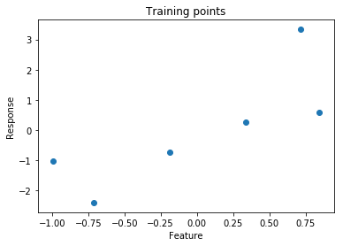
One way to do fit a line to the points would be to minimize the loss function for linear regression, mean squared error, expressed as \(L(\boldsymbol{w};d) = \frac{1}{n}\sum_i(\boldsymbol{y}_i-\boldsymbol{x}_i\boldsymbol{w})^2\). The loss for a single point is the squared error, \((\boldsymbol{y}_i-\boldsymbol{x}_i\boldsymbol{w})^2\). Below is the loss for each point as well as the mean squared error.

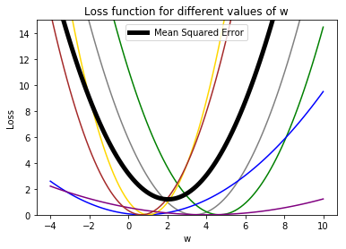
Applying gradient descent in this case looks like:

This visualization could have been rendered without the individual losses and it would still reflect the descent on the mean loss. Gradient descent doesn’t care how your function came to be, just that it can follow the gradient. In contrast, Stochastic gradient descent is going to make use of the individual component loss functions.

Stochastic Gradient Descent (SGD)

Stochastic gradient descent has a similar form as gradient descent but instead of averaging the loss for every training point, SGD randomly selects one point \(d_j\) at each iteration and updates the parameters based on the gradient of that single loss:

\[\boldsymbol{w}_{t+1}=\boldsymbol{w}_t-\alpha\nabla g(\boldsymbol{w}_t;d_j)\]

While iterating, SGD decreases the learning rate; this is crucially important to making sure it converges. SGD stops when the learning rate is sufficiently small or the average loss has converged.

A common variant of SGD is to use a subset of the data on each iteration instead of a single point and average the loss of the subset. These subsets are referred to as mini-batches. The reason for this is discussed in the next section.

I was confused by SGD because instead of minimizing the function you care about, you are randomly picking components and updating based on that component. I was imagining the case where the algorithm is close to optimal on the average loss but unluckily picks a component loss that is far from the average and pushes the parameters way off. How could you trust the algorithm to converge?

Consider the first few iterations of applying SGD to our same data above. Now it is showing both the average loss as well as the loss function selected to determine the gradient.

That looks chaotic, doesn’t it?

Why SGD Works

To understand why SGD works, it is necessary to take a step back and look at what we are really doing when minimize the average loss function:

\[f(\boldsymbol{w}) = \frac{i}{n}\sum_i g(\boldsymbol{w}; d_i)\]

Can be viewed as the expected value of \(g(\boldsymbol{w};d)\) over the empirical distribution of samples, \(d\), i.e., \(f(\boldsymbol{w}) = E_d[g(\boldsymbol{w})]\). We are hoping the distribution of samples we have reflects the true distribution these samples came from and, therefore, our model is good at predicting the true distribution.

Looking at our average loss, \(f(\boldsymbol{w})\), as an expectation gives us a way to understand how SGD works. The average loss of our samples is an estimate of the expected loss of the true distribution. Taking the loss of a single sample is also an estimate of the true expected loss, just likely a worse estimate. Mini-batches often help SGD by providing better estimates of the true expected loss while still containing noise that is helpful for training.

Luckily, in expectation, repeatedly taking the loss of single samples will tend to the expected loss (almost surely). For intuition, consider how many samples will push the parameters in the wrong direction compared to the right direction (and by how much) at each iteration.

For a formal explanation of this, as well as why it is necessary to decay the learning rate, I found Online Learning and Stochastic Approximations by Léon Bottou to be helpful.

The last question you might be thinking is, why would I use SGD over gradient descent? First, SGD requires a lot less computation on each iteration which is helpful when the dataset is very large. Second, SGD tends to work better on non-convex functions because it causes the parameters to jump around more. Both of these properties apply to machine learning problems in the wild.

To end, here is the full run of SGD that we cut off prematurely above (it takes about a minute to converge):

If you liked this post, think I should add something or found an error I should correct, please let me know on Twitter – @wyegelwel.

Acknowledgements

Thank you to Alex Adamson for giving me insight into how SGD works, and thank you to Kat Kennovin and Logan Sorrentino for reviewing early drafts of this post.